This tutorial will introduce you to writing and running simulations using the NepidemiX module and its associated utility scripts.
I advice you to go through the sections in order and do the exercises as they will build you a set of own configuration files and show how to use some of the scripts.
This section lists some very basic concepts that may be good to grasp before starting the actual tutorial. The descriptions are quite brief, and if you feel that the concepts here are somewhat out of your grasp it may be a good idea to look around the web for some additional information before proceeding.
ini files are an old (informal) standard among configuration files. The format is not very flexible, but easy to read and write. The NepidemiX scripts are currently configured using ini files.
The files are pure text files (but usually named with the ending .ini instead of .txt), and the format simple. The file is divided into sections where each section name is written between square brackets. Within a section options are set using the = sign. Comments are written on a line following a # sign. For example:
[Simulation]
# Run the simulation this many iterations
iterations = 500
# The time step taken each iteration
dt = .1
The NepidemiX scripts are terminal programs. That means that they don’t have any graphical user interface, and that you will have to execute them from the command line. I will assume that you know how to open a terminal and how to change directories.
This may not be an issue, but as it may be confusing in case you don’t know the difference between these concepts.
When working in a shell environment one sometimes distinguishes between absolute and relative paths.
Absolute paths are the full search paths on a file system. The path starts in the file system root. Examples:
- C:\Windows\autoexec.bat This is an absolute file path on a windows system.
- /home/lukas/Documents/ An absolute directory path on a *nix system.
Relative paths on the other hand are relative to the current location (the old lingo is where you are standing) of program execution. This is different from where the program itself is located, and mostly correlates where in the directory hierarchy you execute it. Examples:
- Documents\data.xls The file data.xls located the directory Documents which in turn is located in the same directory as we are (windows slashes)
- ./Documents/data.xls The same on a *nix system (with the ./ meaning current directory explicit).
- ../music.mp3 The file music.mp3 located one directory above wherever we are currently located.
Today we usually don’t have to distinguish between relative and absolute paths very often so it can get confusing. When configuring and running NepidemiX software you will occasionally need to specify file paths. You can use either absolute or relative paths. All paths will be relative to the directory where you will be executing the python command.
In the examples below I use relative paths for the simple reason that I do not know where on your file system you will end up saving the files. This is not a problem and quite flexible, but make sure you ‘stand’ in the correct directory when you execute the code, as it will not run otherwise.
Nodes and edges can be associated with attributes. An attribute has a name and a value and will typically describe something about the node/edge. When running a simulation of a process we typically changes these attributes, and we are interested how they evolve over time. An attribute can describe anything, for instance: age, HIV status, or gender. A node/edge can have one or more attributes. The state of a node/edge then is dictionary/vector of all its attribute values. For instance, if there is a node-attribute called status that can have the values of either S (susceptible), I (infected), or R (recovered). We say that the node is in either S, I, or R state dependent on the value of status. For nodes/edges with several attributes each combination of values is a valid state (and the node must be in one of them). For example: in addition to the status attribute, we add another to the node called gender. This attribute can either be male or female. Such a node is in one of six states (S+female, I+female, R+female, S+male, I+male, R+male), all combinations of possible attribute values. Finally, a partial state is what possible state a node can be in given information on none, or some of its attribute values. The concept is used when selecting nodes/edges of certain classes. Thus, if we had nodes with the same two attributes as in the previous example, we could select the nodes in the partial state gender = male. This would match any of the states S+male, I+male, R+male.
First, if you haven’t done so already download and install NepidemiX module as described here Downloading and installing NepidemiX .
If you have done the above steps correctly you will have a directory structure looking something like:
- tutorial/
          - conf/
          - output/
Moreover, you should be able to open a python shell and write:
>> import nepidemix
without getting any error messages.
After the installation you should also have the executable script nepidemix_runsimulation on your system. Open a command prompt and try to run it:
> nepidemix_runsimulation
It should exit after complaining about too few arguments.
Now, we can start running some simulations!
While the nepidemix module can be loaded in an interactive python shell (like all other python) module it was primarily designed to be accessed by applications. To use it interactively would mean that we need to manually load and create an appropriate configuration every time. This is cumbersome, and better scripted. We will use the python program nepidemix_runsimulation for this. In its simplest form the script require one argument: a configuration file. The next step is to write this file.
For our first simulation let’s use a simple, but standard model: the SIS process.
If you are not already familiar with the basics of this process. It has two states, susceptible S and infected I. In a network setting a node can transition to state I (given that it is in state S) with the following probability in unit time  , where
  is the number of neighboring nodes in state I, and
  is the infection rate.
Given that it is already in state I the node can transition to S again with the probability
is the infection rate.
Given that it is already in state I the node can transition to S again with the probability  in unit time.
I will return to the parameters  when configuring the process below, but for now let us start writing the configuration file that will set up the simulation.
Later I’ll show you how to specify processes, but for now let’s use a pre-made SIS specification.
Copy the file SIS_process_def.ini to your config folder. It should be located in examples/tutorial/conf/ in the NepidemiX documentation.
If you can not find the file, or rather want to have a look at the contents, use your favorite text editor to create a file called SIS_process_def.ini it in the config folder and copy the following into it:
[NodeAttributes]
status = S,I

[MeanFieldStates]
{status:S}
{status:I}

[NodeRules]
{status:S} -> {status:I} = NN({status:I}) * beta
{status:I} -> {status:S} = delta
You can probably figure out what most of this definition is by just looking at it, but if there’s anything that seems unclear, don’t worry, we’ll go through process specifications later in Using ScriptedProcess to write node-state-processes.
First, however, I’ll show you how to run the SIS process on a network by writing a simulation configuration file.
So, go ahead and create a new file in your config folder called SIS_example.ini. This will contain the configuration describing our simulation.
Now, let’s fill in SIS_example.ini together.
We start with the following general piece of simulation information:
# This is the simulation section.
[Simulation]
# Run the simulation this many iterations.
iterations = 500

# The time step taken each iteration.
dt = .1
# This is the name of the process object.
process_class = ScriptedProcess

# This is the name of the network generation function.
network_func = barabasi_albert_graph_networkx
The comments behind the # symbols should be fairly self-explanatory. The section title is written in square brackets; the options are to the left of the = signs and whatever is on the right is the value of said option.
Note the option process_class is set to the value ScriptedProcess. The name ScriptedProcess is a class defined within the nepidemix module. The value of process_class determine which process will run on the network. There are no finished processes defined within nepidemix. One can specify processes by either ini scripting or by writing a Python class. Later in this tutorial we’ll see how to define new Processes. ScriptedProcess just means that the process will be provided as a configuration file.
The network generation algorithm function is set using the option network_func. Set it to the value barabasi_albert_graph_networkx which is the networkx implementation of the BA preferential attachment algorithm. There are a few different network generation functions implemented already, for example: grid_2d_graph_networkx – create a regular grid; fast_gnp_random_graph_networkx – Erdős-Rényi random graph; load_network – load a network from file; connected_watts_strogatz_graph_networkx – Watts-Strogatz graph.
The network generation algorithm specified by the network_func option in the Simulation section will typically need some parameters to generate a network (size for example). These are given in the following section called [NetworkParameters]. As different network generation algorithms will need different parameters the actual options of this section will vary. [[NepidemiX (Documentation)]] has a section describing the implemented network generation functions and what configuration options they require. For now, we will go with the BA preferential attachment, and this implementation needs two options. n – the number of nodes in the network, and m – the number of edges to preferentially attach to a new node when growing the network. Now, update your settings file by adding the following:
# Network settings.
[NetworkParameters]
# Number of nodes.
n = 1000
# Number of edges to add in each iteration.
m = 2
For this example we will use a rather small network, 1000 nodes, but if you like you can later change this value to run the simulation on larger (or smaller) networks.
This section serves two purposes: to tell the simulation which process script we want to use, and to define any process parameters in that script.
The file option in the configuration section below is the name of the process definition file. In our case it is SIS_process_def.ini.
The process parameters are the parameter values in our process model. They options in this section must match the names for the process parameters. When implementing custom processes later we’ll see how to define the parameter names. For the already defined SISProcess however we have the two parameters beta and delta (corresponding to , delta in the process description) so this needs to be the name of the options given here.
Copy the following into your SIS_example.ini file:
# Defining the process parameter values.
# The contents of this section is dependent on
# the parameters of the process class as specified by
# the option process_class in the Simulation section.
[ProcessParameters]
# File name of the process description.
file = SIS_process_def.ini
# Infection rate.
beta = .9e-2
# Death rate.
delta = 0.0076
As a note, the values have been picked mostly at random from another test project. Assuming that one iteration is one month we use an infection rate of 0.09, and an average survival time of about 11 years ( ). Feel free to try out your own values if you like.
This section considers the initial distribution of states among the nodes of the network. The section header is [NodeStateDistribution] and the name of the options depends on the configured process in the following way. They must correspond to the names of the states used by the Process implementation! For the SISProcess in this example the state names are {status:S} and {status:I}. Later when you define your own processes you can of course chose whatever state names you like. Update your SIS_example.ini file with the following section:
# The fraction of nodes, alternatively the number of nodes, that will be  assigned to each state initially.
# The state names must match those specified by the network process class.
[NodeStateDistribution]
# 95% S
{status:S} = 0.95
# 5% I
{status:I} = 0.05
The value of the state options must be a number. If the sum of the states add up to the size of the network the exact number of nodes will be used. If not a fraction of the network equal to the (network size x state dist)/(sum of all state dist) will be used. I.e. normalized. It is recommended to either use exact numbers or fractions of the network size here for readability.
The NodeStateDistribution section is optional. If this section is left out an equal number of nodes are allocated to each state.
Finally, we must define what data should be saved, where it should be saved, and what it should be called. Update your configuration file with the following:
# Result output settings.
[Output]

# Output directory:
output_dir = ../output/

# This is the base name of all files generated by the run.
base_name = test_SIS

# If unique is defined as true, yes, 1, or on, unique file names will be created (time stamp added)
unique = yes

# If this is true, yes, 1, or on, a copy of the full program config, plus an Info
# section will be saved.
save_config = yes

# If this is true/yes/on, the network node states will be counted and saved as a csv file.
# Default value True.
# Note only valid if the current process support updates. If not nothing will be saved.
save_state_count = yes

# Count nodes every ... iterations. Value should be integer >= 1.
# Default value 1.
save_state_count_interval = 1

# If this is true, yes, 1, or on, a copy of the network will be saved.
# Save interval may be set using the save_network_interval key.
save_network = yes

# This control how often the network will be saved.
# A value <= 0 means only the initial network will be saved. A positive value
# n> 0, results in the initial network being saved plus every n:th iteration
# thereafter, as well as the last network.
# Default value 0.
save_network_interval = 0
I have kept the rather extensive comments in this part of the configuration as they can good for remembering what is going on. The options should be quite self-explanatory from the comments, however I want to point out a few things. First the value of the option base_name will be the prefix of all saved files. Second, the value of output_dir should be an existing directory. All files will be saved here. Note also that the value in this particular example is a relative path, ../output/. You can use the absolute path to your output directory if you like, but as this tutorial should be general I will use a relative path here. Using a relative path however does mean that when we run the simulation it will try to save the data in a directory called output located one level up from where the simulation is executed - we must therefore take some caution to where we will run our simulations. See below.
You should now have the file SIS_example.ini all filled in and saved in your conf directory. We are ready to execute our simulation! Exciting!
Open a command line prompt in the conf directory. We will execute the simulation from here (as we are using relative paths).
Run the simulation:
> nepidemix_runsimulation SIS_example.ini
Anyway, after pressing return the simulation will print a lot of things and hopefully run to an end. Depending on your settings and computer you will now have time to blink, wash the dishes, or go for a run. (With the above settings I had just time to brush half of my teeth. Not to self: double number of iterations for next version of the tutorial.)
When the simulation is done and you return to screen have a look in your output directory. If all have gone well you will find four files there: test_SIS_<date>_0000000000.gpickle.bz2, test_SIS_<date>_0000000500.gpickle.bz2, test_SIS_<date>_2011.ini, test_SIS_<date>_state_count.csv . Where <date> is the date and time of execution. So what are these files?
In fact, go ahead and do what is suggested in the last bullet point above: look at the csv file. Either in a text editor or by importing in in a spread sheet application. You’ll see three column headings Time, frozenset([(‘status’, ‘S’)]), and frozenset([(‘status’, ‘I’)]). The Time column is the current iteration times the time step (dt). The other two columns has quite funny names, but if you ignore the frozenset text and the brackets, it is quite easy to imagine that this is the nodes which has status S and I respectively. This is also the case. The two columns contain the number of nodes in each state. As you can see there are 950 S nodes to start with and only 50 infected.
To visualize how the numbers change over time you can easily make a scatter plot with Time on the horizontal axis and the node counts on the vertical. It should look something like this:
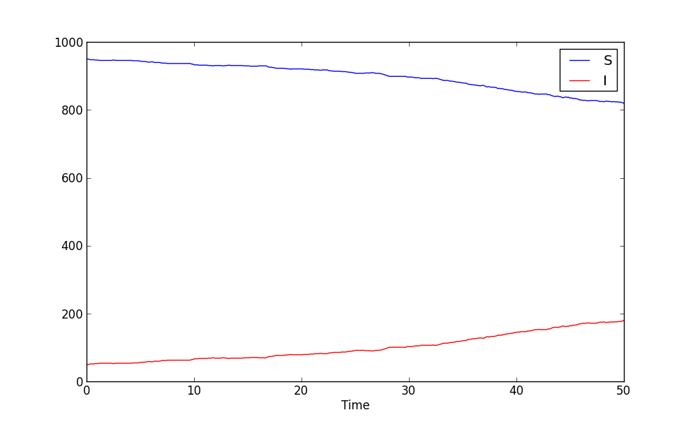
As you can see the Susceptible population is in decline while the Infected is rising. But is this how it will end? Clearly the simulation has not been run enough time steps. Go ahead and increase it! How long do you have to run it before you are reasonably sure to have reached a steady state?
You probably know this, but as a side note: in reality, running a single simulation will not be enough as they are stochastic. You will need to run a lot of them and average the results.
Now, take some time now to play around with some of the parameters, for instance increase the number of iterations, network size, and try some different values of beta and delta. Plot the data in the csv file.
When you are done we’ll define an SIR process.
OK, so the SIS process was fun, but how do we describe our own?
There are currently two ways to build processes for a nepidemix simulation to use. The first is to script it using a specific type of ini file, and the second is to program a custom Python class. This section consider the first option. It is not quite as flexible as when writing your own python code of course but can go a long way for many node-state simulations.
Use this approach if your process
Here we’ll look at the SIR process. S – susceptible, I – infected, and R – recovered. That is instead of dying after some time in the infected class and returning to susceptible (the SIS model), the node recover and end up in the R state.
We will let the rate of infection be , and the recovery rate be  . The transition probabilities in unit tile are then
, where is the number of neighbors in state I.NepidemiX has the functionality to turn these type of transition rules into the python code for a process. All that is needed is a specifically written configuration file. Let’s start! Open a new file called SIR_process_def.ini in your editor and copy the following into it:
[NodeAttributes]
status = S,I,R
The section NodeAttributes is used to declare the name and possible values of all node attributes. The above line lets the program know that there is one attribute called status and that it can have one of the three values S, I, R. You could have chosen other names if you had liked. Note that nodes may have many different attributes (for instance we may have one called gender, and another called age) they would all be declared on separate rows in the NodeAttributes section followed by their possible values. Note that nepidemix require a finite number of possible values for an attribute, meaning that each one has to be declared. For the example age that could have quite many different values the range short hand <start>:<step>:<end> would have been the easiest choice, e.g age = 0:1:150 for an age between 0 and 149.
In short the NodeAttributes section lets you declare the names and symbols used to define an attribute. But now back to our SIR process.
Next we need to define the mean field states. We would not have to declare any states here, as the SIR model do not have any transition rules dependent on the mean fields, however the simulation software will log how many nodes are in the declared mean field states progress over time. This is what you see in the ‘frozenset’-columns in the resulting csv file. There will be one column for each declared state. Thus by declaring all three states we make sure that we will have data saved for them.
Write the following section in your configuration:
[MeanFieldStates]
{status:S}
{status:I}
{status:R}
As you can see, the mean field states is not an assignment, but just a list. You write the state between curly brackets on the form { <attribute1>:<value1>, <attribute2>:<value2> }. The state can be full or partial (as described in Lingo: states, partial states, and attributes). If it is a partial state the simulation will automatically insert all possible full states matched by this state. To match all possible states use the most general partial state: {}. (If you, like you can insert that state as well in the definition. Do you know what you would get?)
Next up is declaration of the actual rules; add the following to the file:
[NodeRules]
{status:S} -> {status:I} = NN({status:I}) * beta
{status:I} -> {status:R} = gamma
Save the file as SIR_process_def.ini in the conf directory.
Worth noting in the above configuration is that the rules must have a specific form.
The options must be on the form <Source state> -> <State update>
- A state such as <Source state> is written as a dictionary of node attributes on the form. {<attribute1>: <value>, <attribute2>: <value> ...}. Partial states ( as described in Lingo: states, partial states, and attributes ) can be used.
- The <State update> is written as a partial state only listing the changed attributes and their new value.
The values of the options must be an expression computing the probability (in unit time) for the state transition.
- NN is a built-in function that returns the number of nearest neighbor in some state.
- All symbols not arithmetic, states, or defined functions (currently NN for nearest neighbors, and MF for mean field) are treated as parameters. Their values will be defined below.
Name parameters and state names using strings. Anything that is OK in a python interpreter should be OK here. Stay away from python’s reserved words.
Thus, when reading the above configuration network model will create a custom process with the states found on the options side (left hand of the = -sign) and with the parameters found on the value side (right hand side of the = -sign). It has no way of knowing the values of the parameters, nor the initial state distribution of the network. That is why we need the same kind of configuration file as for the SIS example above in order to run the simulation.
I’m going to assume that you have done that part of the tutorial and have a pretty good idea about what the different configuration options mean already. Therefore, I will only point out the differences used for the SIR model. Copy the below into a new file and save it as SIR_example.ini in the conf directory:
# This is the simulation section.
[Simulation]
# Run the simulation this many iterations.
iterations = 500

# The time step taken each iteration.
dt = .1

# This is the name of the process object.
process_class = ScriptedProcess

# This is the name of the network generation function.
network_func = barabasi_albert_graph_networkx

# Network settings.
[NetworkParameters]
# Number of nodes.
n = 1000
# Number of edges to add in each iteration.
m = 2

# Defining the process parameter values.
# The contents of this section is dependent on
# the parameters of the process class as specified by
# the option process_class in the Simulation section.
[ProcessParameters]
# File name of the process description.
file = SIR_process_def.ini
# Infection rate.
beta = .9e-2
# Recovery rate.
gamma = 0.04

# The fraction of nodes, alternatively the number of nodes, that will be  assigned to each state initially.
# The state names must match those specified by the network process class.
[NodeStateDistribution]
# 95% S
{status:S} = 0.95
# 5% I
{status:I} = 0.05
# Zero recovered to start with.
{status:R} = 0

# Result output settings.
[Output]

# Output directory:
output_dir = ../output/

# This is the base name of all files generated by the run.
base_name = test_SIR

# If unique is defined as true, yes, 1, or on, unique file names will be created (time stamp added)
unique = yes

# If this is true, yes, 1, or on, a copy of the full program config, plus an Info
# section will be saved.
save_config = yes

# If this is true/yes/on, the network node states will be sampled and saved as a csv file.
# Default value True.
# Note only valid if the current process support node updates. If not nothing will be saved.
save_node_state = yes

# Sample node every ... iterations. Value should be integer >= 1.
# Default value 1.
save_node_state_interval = 1

# Sample node every ... iterations. Value should be integer >= 1.
# Default value 1.
save_node_state_interval = 1

# If this is true, yes, 1, or on, a copy of the network will be saved.
# Save interval may be set using the save_network_interval key.
save_network = yes

# This control how often the network will be saved.
# A value <= 0 means only the initial network will be saved. A positive value
# n> 0, results in the initial network being saved plus every n:th iteration
# thereafter, as well as the last network.
# Default value 0.
save_network_interval = 0
What changes can you see in this configuration compared to the one you used in the SIS example? There are not many
Let’s start with the easiest one. I changed the base_name option under [Output] to reflect that we are now running a SIR process.
However, as the process has changed so must the configuration options in the section dependent on it.
As we know since before the option in [ProcessParameters] must correspond to those accepted by the process class. For ScriptedProcess this is
- Always an option called file. The value of this option is the name (and path) of the file where we saved the transition rules. In our case the value is SIR_process_def.ini (and we can skip the path as it is saved in the same directory as where we will run the simulation [ not because it is in the same directory as the simulation config file]).
- Whatever process parameters used in the process definition file. In our case this is beta and gamma as these are unknowns in our right hand transition rate specifications.
The choice of process also influence the [NodeStateDistribution] section. Remember that this section contains one option per state defined by the process, and the states are defined by the left hand sides in SIR_process_def.ini. There are three different state names being used: {status:S}, {status:I}, {status:R} - their initial rates must be set.
That is it. From the conf directory - run the simulation:
> nepidemix_runsimulation SIR_example.ini
When the simulation is finished you’ll find the same kind of files in your output directory as after the SIS simulation, but now prefixed by the new base name.
Why don’t you take the contents of the csv file and plot the state counts of the S, I, R states? Anything interesting in there? You will probably discover that you need more iterations, so go ahead and increase it, run another simulation, get a cup of tea, and plot it again.
Here are a couple of things to try out
In some cases the ability to state simple rules is not enough for a process and we can not use the ScriptedProcess. In this case the process needs to be implemented as a python class.
All processes are children of the top class nepidemix.process.Process, and thus need to define the appropriate methods from its interface. To simplify matter we can also derive processes from one of the subclasses ExplicitStateProcess, or AttributeStateProcess.
ExplicitStateProcess represents methods who’s node and edge states are explicitly stated in each node. That is, unlike our scripted representation where a state was a unique combination of attribute values, this class stores just the name, or enumeration of the state. For instance, status=S could be called ‘S’, and status=I called ‘I’.
For a similar treatment of states as the ScriptedProcess above before, we could also derive from AttributeStateProcess which has some methods implemented when we want to treat the state as a combination of attribute values.
In the following example we will be using ExplicitStateProcess and define the way node states are updated. We will start by re-implementing the SIR model as a python class.
Note: ExplicitStateProcess does not care about attributes (or rather only about a single attribute, the state) and therefore you do not need to care about the attribute/state/partial state -notation we used with the ScriptedProcess. A state is just a string (a single symbol). This makes notation easier but is not as powerful as before.
As we saw above the SIR process can be scripted without doing any python programming. However, as we are already familiar with this model let’s start by writing it as a python class.
Under your tutorial directory create a new directory and name it modules. In this folder open a new file called extended_SIR.py. We will write our python classes in this file.
At the top of the file we will first import some external modules that we will need:
from nepidemix.process import ExplicitStateProcess
from nepidemix.utilities.networkxtra import attributeCount, neighbors_data_iter
import numpy
The first two lines import the ExplicitStateProcess class from nepidemix as well as a utility functions, NepidemiX-API-networkxtra.attributeCount, (useful to count attributes on networkx graphs) and NepidemiX-API-networkxtra.neighbors_data_iter (yielding an iterator over nearest neighbors in a networkx graph, together with their attribute dictionaries) . The third line imports the numpy package.
Now we are ready to derive a class for the SIR process. Classes in python are defined using the class keyword, so go ahead and declare a class called SIRProcess deriving from ExplicitStateProcess, the code looks like this:
class SIRProcess(ExplicitStateProcess):
This by itself isn’t very much, we must also fill in the methods that we wish the simulation to use. One method that is always needed is the in python specially named __init__ - called whenever an instance of the class is created. Its purpose is to initialize the process. The second method we will need is called nodeUpdateRule. This method is defined in the Process class and will be called once per node per iteration. It is responsible for updating the state of a node.
Now update your code so that it reads:
class SIRProcess(ExplicitStateProcess):
    def __init__(self, beta, gamma):
        pass

    def nodeUpdateRule(self, node, srcNetwork, dt):
        pass
This code only declare the class and the methods. The pass command just tells python that nothing is being done (I’ve put there so that your programming editors won’t be confused by empty declarations).
As you can see I have listed the parameters of the methods. The first parameter in a class methods must always be self which when the method is being called will be a reference to the instance of the class calling the method. Thus self is akin to this used in C++ and Java, however it is explicitly listed as a parameter in python.
Now, let’s look at the other parameters passed into the methods. __init__ takes two parameters: beta and gamma, these will represent the infection and recovery rates respectively. (We used the same names for the rates in the scripted example above, remember?). The important thing to remember here is that whatever parameters we name here (except for self) needs to be defined as options in the ProcessParameters section of the simulation configuration file. I will return to this.
The nodeUpdateRule then is declared to accept three parameters: node, srcNetwork, and dt. This is how the simulation will call it to request an update of a node. node is a reference to a NetworkX node, and Simulation expects nodeUpdateRule to decide if the state of the node should be updated, and if so what the new state should be. Finally the method should update the state of node and also return it. The parameter srcNetwork is the full NetworkX graph at the state of the previous iteration. It should be read from! A node update rule method must only make changes to the current node, as anything else will skew the simulation. dt, finally, is the time step since last iteration.
Now that we know what information is being passed to the methods we can go ahead and implement them. First, __init__:
def __init__(self, beta, gamma):

   super(SIRProcess, self).__init__(['S', 'I', 'R'],
                                    [],
                                    runNodeUpdate = True,
                                    runEdgeUpdate = False,
                                    runNetworkUpdate = False,
                                    constantTopology = True)
   self.beta = float(beta)
   self.gamma = float(gamma)
As you can see, I have gone ahead and replace the pass with a few lines of code. You can go ahead and do the same in your file. When you are done I’ll tell you what the code does.
The only piece of code here that may seem a bit mysterious is the first call super... and so on. What it does however is really simple: it calls the __init__ method of our super class. Which is ExplicitStateProcess as we derived from that class. The reason why we need to do this is that there may be code (there is!) in that class that needs to be executed when the class instance is created. Remember, our SIRProcess is an ExplicitStateProcess and thus share that class’ attributes. (Maybe you now think, well, it’s also a Process class, what about that initialization? The answer is that as it is not a direct descendant we don’t need to worry; ExplicitStateProcess will take care of that. But in theory you are correct.) The command super will, given a class name, and a class instance (self) yield the super class of said class. After that we may call the __init__ method of said class as if it was called from our SIRProcess object.
Anyway, to figure out what parameters we should send, go ahead and have a look at the documentation for ExplicitStateProcess by clicking that link, or use the pydoc utility:
> pydoc nepidemix.process.ExplicitStateProcess
We can see that its init-method has the following form __init__(self, nodeStates, edgeStates, runNodeUpdate=True, runEdgeUpdate=True, runNetworkUpdate=True, constantTopology=False). Except for the self-parameter (which will be automatically filled in by python, so we don’t have to worry about it) it takes five arguments. The first two, nodeStates and edgeStates are lists containing the node and edge state names respectively. This explain the first two parameters in the super call: the first list contain the names of node states, S, I, R. The second is an empty list because this model does not have any node states. Finally, there are three Boolean valued variables. In the definition these all have standard values set to true: runNodeUpdate=True, runEdgeUpdate=True, runNetworkUpdate=True (this means that if we would not send in any parameters here they would get these values). The flags will tell our simulation if it should try to do node, edge, and network state updates respectively. (A network update is an update to attributes associated with the network as a whole.) As I wrote, by default these are all on, however, as our method only has node updates, and we do not care about edge or network updates we may set the last two to false. The same goes for the last flag, constantTopology, by setting this to True the Simulation will know that your process does not change any network topology. This will speed up the simulation as it may skip these steps.
The last two lines of code in the example above, creates two class attributes in the SIRProcess class called beta and gamma, and assigns to them the value of the parameters beta and gamma that was sent in to the init method. Before assignment the parameters are converted to float type. This is because we can not be sure what type the sent in parameters will have (actually they will mostly be strings as they are read from the setup files which are text) and thus we need to try to convert them.
And now on the interesting stuff: nodeUpdateRule, taking care of the state updates is implemented like this:
def nodeUpdateRule(self, node, srcNetwork, dt):
     # Read original node state.
     srcState = node[1][self.STATE_ATTR_NAME]
     # By default we have not changed states, so set
     # the destination state to be the same as the source state.
     dstState = srcState

     # Start out with a dictionary of zero neighbors in each state.
     nNSt = dict(zip(self.nodeStateIds,[0]*len(self.nodeStateIds)))
     # Calculate the actual numbers and update dictionary.
     nNSt.update(attributeCount(neighbors_data_iter(srcNetwork, node[0]),
                 self.STATE_ATTR_NAME))

     # Pick a random number.
     eventp = numpy.random.random_sample()
     # Go through each state name, and chose an action.
     if srcState == 'S':
         if eventp < self.beta*nNSt['I']*dt:
             dstState = 'I'
     elif srcState == 'I':
         if eventp < self.gamma*dt:
             dstState = 'R'

     node[1][self.STATE_ATTR_NAME] = dstState

     return node
I have left some comments in the above code to highlight what is happening. I will explain some of them.
First node[1][self.STATE_ATTR_NAME], remember that node is a NetworkX node. Thus it will be a pair on the form (<node id>, <attribute dict>). So, node[1] gives us the dictionary, and the following [self.STATE_ATTR_NAME] simply look up the attribute named with the value of self.STATE_ATTR_NAME. Which, as we have derived from ExplicitStateProcess is the state.
Second, there is a couple of lines looking like:
# Start out with a dictionary of zero neighbors in each state.
nNSt = dict(zip(self.nodeStateIds,[0]*len(self.nodeStateIds)))
# Calculate the actual numbers and update dictionary.
nNSt.update(attributeCount(neighbors_data_iter(srcNetwork, node[0]),
                           self.STATE_ATTR_NAME))
dict(zip(self.nodeStateIds,[0]*len(self.nodeStateIds))) may look complicated, but what it does is to construct a python dictionary where they keys are state names and where the values are zero. zip is a python function that takes two lists and interleave their values as tuples in a new list (which then dict coverts to a dictionary). The lists we send in to this is first the list of node states, named nodeStateIds. Now you may say ‘hey, I did not construct that attribute of the SIRProcess class! No, you did not, but the call of the init-method of its superclass ExplicitStateProcess did. You probably saw this mentioned in the pydoc documentation of that class.
So, now we have a dictionary of counters for every state a node can be in, what do we do with it? Well the next line will count the number of nearest neighbors of the node and update the dictionary with this value. NepidemiX-API-networkxtra.attributeCount is a utility function that can be found in nepidemix.utilities.networkxtra (check it out with pydoc if you like). It accepts two parameters: first an iterator over all nodes with data that should be counted (this could be an iterator over the full network, or in this case just over a subset) and the name of the attribute to count (in this case the name of the attribute holding the node state).
Finally, let me explain the call neighbors_data_iter(srcNetwork, node[0]). This is also a nepidemix utility function and it creates an iterator over the nearest neighbor node, data-tuples given a network and a node in this network. Remember that srcNetwork is the NetworkX graph sent to our method and node[0] is the node ID in this network. You may ask why we need a utility function to build this iterator, doesn’t NetworkX provide functions for this? Unfortunately not in this case: the nearest neighbor iterator provided by NetworkX does only give an iterator over node id’s and not over (<id>, <data dict>) tuples, which is what is needed in this case.
Long explanations, but fortunately you will most probably not need to change any of this particular piece of code in your own implementations.
Now that we know the state of our node and have a dictionary where we can look up the number of nearest neighbors in a specific state, we are ready to check if the state of the node should be changed.
First a random number between 0 and 1 is created using one of numpy’s random functions. This is our event. We then check what this event will mean given what state the current node is in this is the nested if-cases following:
# Go through each state name, and chose an action.
if srcState == 'S':
    if eventp < self.beta*nNSt['I']*dt:
        dstState = 'I'
elif srcState == 'I':
    if eventp < self.gamma*dt:
        dstState = 'R'
You can see us checking the variable srcState first and in case we are in that state computing a probability to compare our event to given that we are in that state. The attributes self.beta and self.gamma that were set in the __init__ method are used here. Also not that the computed probabilities are multiplied with dt as the formulas given for the SIR model above were in unit time (0 < dt <=1 [typically]).
The final two rows of the method implementation respectively sets the state attribute in the node attribute dictionary to whatever value is in dstState (if none of the events happened in our if-cases this value will be the original state and nothing happens), and returns the node. These two rows are important as without them the simulation might run but not much would happen.
Now, then, to repeat, you should have something like the following in your editor:
from nepidemix.process import ExplicitStateProcess

from nepidemix.utilities.networkxtra import attributeCount, neighbors_data_iter

import numpy


class SIRProcess(ExplicitStateProcess):
    """
    S I R process,

    Attributes
    ----------
    beta - Infection rate.
    gamma - Recovery rate.
    """
    def __init__(self, beta, gamma):

        super(SIRProcess, self).__init__(['S', 'I', 'R'],
                                         [],
                                         runNodeUpdate = True,
                                         runEdgeUpdate = False,
                                         runNetworkUpdate = False,
                                         constantTopology = True)
        self.beta = float(beta)
        self.gamma = float(gamma)


    def nodeUpdateRule(self, node, srcNetwork, dt):
        # Read original node state.
        srcState = node[1][self.STATE_ATTR_NAME]
        # By default we have not changed states, so set
        # the destination state to be the same as the source state.
        dstState = srcState

        # Start out with a dictionary of zero neighbors in each state.
        nNSt = dict(zip(self.nodeStateIds,[0]*len(self.nodeStateIds)))
        # Calculate the actual numbers and update dictionary.
        nNSt.update(attributeCount(neighbors_data_iter(srcNetwork, node[0]),
                                   self.STATE_ATTR_NAME))

        # Pick a random number.
        eventp = numpy.random.random_sample()
        # Go through each state name, and chose an action.
        if srcState == 'S':
            if eventp < self.beta*nNSt['I']*dt:
                dstState = 'I'
        elif srcState == 'I':
            if eventp < self.gamma*dt:
                dstState = 'R'

        node[1][self.STATE_ATTR_NAME] = dstState

        return node
This is the full class implementation and we are ready for a first test run.
To run a test we will of course need a configuration file, open up the configuration file you used for the scripted SIR process earlier and save it under a new name (as I am running out of imagination I picked the fantastic name SIR_example2.ini). You may leave most of the settings unchanged, but we will need to make a few changes to a couple of sections. Let’s start with the [Simulation] section. First, change the value of the process_class option:
# This is the name of the process object.
process_class = SIRProcess
It is now set to SIRProcess, the name of the class we just wrote. However, as this class is not part of NepidemiX we also need to tell the simulation where to find it. This is done by adding the following options:
# This is the python module containing the process we wish to use.
process_class_module = extended_SIR

# We need to add another module path
module_paths = ../modules/
If we start from the end, module_paths let’s you tell the simulation where to look for additional python packages and modules that may not be in the standard path. In our case we want to look in the modules directory where we have saved extended_SIR.py. The value of the class module will be extended_SIR (i.e. the file name without the .py ending) which is what we’ll assign to the module_paths option.
When you have changed these options, you can also change the base_name option in the Output section if you want the results to be saved under a different name.
Next, have a look at the ProcessParameters section. With ScriptedProcess we needed to provide the file name of the process definition file. This is no longer needed, so the file option can be removed (but we need to set the values of the unknowns: beta, and gamma.)
Finally, as we are using ExplicitStateProcess as a base for SIRProcess the node names are now the state names: ‘S’, ‘I’, and ‘R’. Thus the NodeStateDistribution section will need to be changed to match the new names:
[NodeStateDistribution]
# 95% S
S = 0.95
# 5% I
I = 0.05
# Zero recovered to start with.
R = 0
Wen you are done with the changes save the file and open a terminal in your tutorial/conf directory. Run the simulation:
> nepidemix_runsimulation SIR_example2.ini
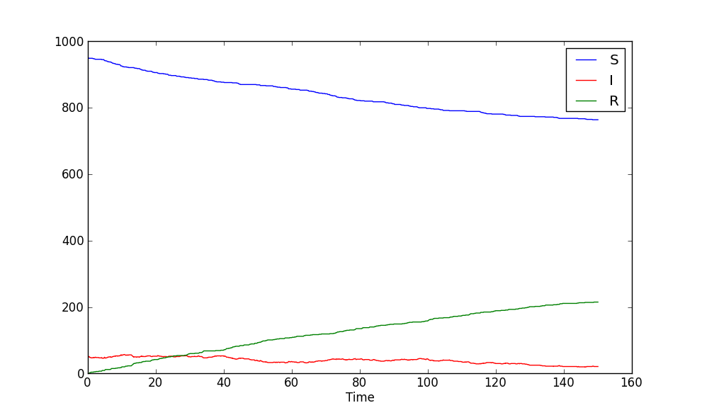
When the simulation is finished compare with the results from the scripted implementation of the SIR process. Do they produce similar results?
This is what a run gave for me over 1500 iterations:
So, now you know how to implement the SIR process in python, but of course we could just as well have scripted that process. I am going to give you a second, slightly more complex example as well.
Let’s extend the SIR model by adding super-spreaders to the infected class. A super-spreader is an infected node who due to some social factors may infect susceptible in the whole population, and not only among their nearest neighbors.
Let us assume that with rate  an infected node turns into a super-spreader; moreover once the node is super-spreading it can not go back to a ‘normal’ infected node. Like all other infected nodes a super-spreader can still recover, however (for simplicity, we assume the same rate, as for the normal infected nodes). As for the additional risk of having super spreaders in the network I will use the naive view that for a single susceptible node the transition probability per unit time to an infected state increases with the fraction of super-spreaders on the network.
Now, there are several way in which we can implement super spreading, a) we could change network topology and link a super-spreader node to all other nodes (or at least all susceptible nodes), or b) we could add a flag-attribute to super-spreader nodes and thus treat them differently, or c) we can add an additional state for infected nodes that is super-spreading. I am sure you can come up with other options as well.
I have chosen to implement c) here, because topology changes may be costly and because I want to keep track of the number of super-spreaders. Let’s call the super-spreader state J, and our new model the SIJR process. Let the transition diagram be the following:
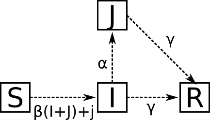
Compared to the SIR process the transition from S to I is now dependent both on the number of infected neighbors ( ) and the fraction of the population in super-spreader-state
  . This implicitly assumes that a node in state J can both spread through normal nearest neighbor contact and through their role as super-spreaders. This can be discussed, but let’s assume it for the purpose of this tutorial.
With that out of the way, let’s do some programming!
Will continue to work in the file extended_SIR.py that you created previously. A python file can contain several classes. Start by creating a class called SIJRProcess in your file, just as for SIRProcess it will inherit ExplicitStateProcess
I will show you the init and node update methods in a little while, but let’s start with computing fraction of the population in state J because what makes the SIJR process impossible to implement using the current ScriptedProcess is that we need access to the fraction of nodes in state J when updating the node states.
Thus, we need to implement it as a python class. Again, there are different strategies to do this, but I will make use of the network update method provided by the Process class. This method, called networkUpdateRule, is called once after all nodes and edges of a network has been updated. The method is given the full network and is free to make any updates to it. We will use this method to set a network attribute that we shall call fracJ representing the fraction of nodes in state J on the network in each iteration.
The most straight forward way of implementing the method is as follows:
def networkUpdateRule(self, network):
    d = attributeCount(network.nodes_iter(data=True),self.STATE_ATTR_NAME)
    network.graph['fracJ'] = d.get('J',0)/float(len(network))
    return network
This implementation relies on the same utility function, NepidemiX-API-networkxtra.attributeCount that we were using in the SIR implementation to get the nearest neighbors, but instead of feeding it an iterator of the nearest neighbors we enter an iterator over all the nodes in the network. The state counts are then stored in the dictionary d, and we query it for the number in state J (telling get to use the value of 0 in case d does not contain the key), dividing this amount by the size of the network.
This will work and run fine, however we explicitly go through all nodes in the network only to count the states, this can be expensive for large networks. Instead we can keep track of the number of nodes in state J when we update the states. Then we will have the number directly in this method and do not have perform the count. The new version of the method would look like this:
def networkUpdateRule(self, network):
    network.graph['fracJ'] = self.Jcounter/float(len(network))
    return network
This assumes that we have a counter called Jcounter in our class with the correct number of nodes in state J. To do so we need to add one to the counter every time a node enters state J and remove one every time a node exits. This will of course be done in the node update rule, so let’s have a look at the implementation:
def nodeUpdateRule(self, node, srcNetwork, dt):

    # Read original node state.
    srcState = node[1][self.STATE_ATTR_NAME]
    # By default we have not changed states, so set
    # the destination state to be the same as the source state.
    dstState = srcState

    # Start out with a dictionary of zero neighbors in each state.
    nNSt = dict(zip(self.nodeStateIds,[0]*len(self.nodeStateIds)))
    # Calculate the actual numbers and update dictionary.
    nNSt.update(attributeCount(neighbors_data_iter(srcNetwork, node[0]),
                               self.STATE_ATTR_NAME))

    # Pick a random number.
    eventp = numpy.random.random_sample()
    # Go through each state name, and chose an action.
    if srcState == 'S':
        if eventp < ( self.beta*(nNSt['I'] +nNSt['J']) + srcNetwork.graph['fracJ'])*dt:
            dstState = 'I'
    elif srcState == 'I':
        # Check recovery before super spreader.
        if eventp < self.gamma*dt:
            dstState = 'R'
        elif eventp - self.gamma*dt < self.alpha*dt:
            dstState = 'J'
            self.Jcounter += 1
        # Super spreaders are still infected and can recover.
    elif srcState == 'J':
        if eventp < self.gamma*dt:
           dstState = 'R'
           self.Jcounter -= 1

    node[1][self.STATE_ATTR_NAME] = dstState

    return node
The form should be familiar to you from implementing the SIR process. Note the increment of the Jcounter when we enter the state from I and the decreasing when leaving from J. Another detail worth thinking about is the branching within the I state where we first check if the node recovers (R), and if not checks if it becomes a super-spreader (J). This does make sense as if the check was in the other order the node could ‘avoid’ recovery by turning into a super-spreader. Finally, look at the transition probability computation going from S to I. Note how the network attribute is used.
There is one piece missing from our counter-puzzle however: the initial count. We can not use 0, because when we run the simulation we can set any distribution in the NodeStateDistribution section. Thus, we have to perform a count after the node states has been initialized. To do so we will overload another method from Process: initializeNetworkNodes. This is the method that the simulation will give the node distribution from the settings and it is responsible for portioning nodes conforming to said distribution out on the network. This functionality is implemented in our parent class ( ExplicitStateProcess ), and we don’t want to re-do that job. Therefore we will overload the method here, then call the original implementation, and afterwards do our own thing. It looks like this:
def initializeNetworkNodes(self, network, *args, **kwargs):
    # Use most of the functionality in the superclass.
    super(SIJRProcess, self).initializeNetworkNodes(network, *args, **kwargs)
    # Now the network should be initialized so we can compute the right fraction of super-spreaders.
    d = attributeCount(network.nodes_iter(data=True), self.STATE_ATTR_NAME)
    self.Jcounter = d.get('J',0.0)
    network.graph['fracJ'] = self.Jcounter/float(len(network))
    return network
Very straightforward, and using elements you have already seen: the super function for reaching into our parent and using its method as if it were our own, and then the same NepidemiX-API-networkxtra.attributeCount code I used in the first example on how to count the states. This time we can’t get around using it, but it is only a single time when the network is initialized so it does not matter.
One thing worth mentioning is the new python formulation *args, and **kwargs. This is simply python’s way of expressing an arbitrary parameter list. *args means unnamed parameters, and **kwargs means named parameters. The result is that the method expects only one argument (network), but that it may be followed by anything. The only thing I do with those parameters is to send them on to the parent class implementation without worrying about what they are. (In practice only the **kwargs part will be used, as the simulation will pass in any thing in the configuration here, and the configuration options must be named, but anyway...)
Only one method to go now! __init__ - and it will look very familiar to you:
def __init__(self, beta, gamma, alpha):

    super(SIJRProcess, self).__init__(['S', 'I', 'J', 'R'],
                                        [],
                                        runNodeUpdate = True,
                                        runEdgeUpdate = False,
                                        runNetworkUpdate = True)
    self.beta = float(beta)
    self.gamma = float(gamma)
    self.alpha = float(alpha)
Note the extended state list (J is in there now), as well as the additional parameter alpha. There is one very small, but also very important change from SIRProcess however: runNetworkUpdate is set to True. If this was not the case networkUpdateRule would not be called and the fraction in state J would forever remain the same, even if the number of nodes in state J may change. (Try it and see!)
That is it, below is the full code for the class, in case you want to control it:
class SIJRProcess(ExplicitStateProcess):
    """
    S I (J) R process, where J is a super-spreader state of the Infected class.
    For simplicity we assume that the recovery rate of the J class is the same
(gamma) as for the I class.

    Attributes
    ----------
    beta - Infection rate.
    gamma - Recovery rate.
    alpha - Rate at which an infected node turns into a super-spreader.
    """
    def __init__(self, beta, gamma, alpha):

        super(SIJRProcess, self).__init__(['S', 'I', 'J', 'R'],
                                            [],
                                          runNodeUpdate = True,
                                          runEdgeUpdate = False,
                                          runNetworkUpdate = True,
                                          constantTopology = True)
        self.beta = float(beta)
        self.gamma = float(gamma)
        self.alpha = float(alpha)


    def nodeUpdateRule(self, node, srcNetwork, dt):

        # Read original node state.
        srcState = node[1][self.STATE_ATTR_NAME]
        # By default we have not changed states, so set
        # the destination state to be the same as the source state.
        dstState = srcState

        # Start out with a dictionary of zero neighbors in each state.
        nNSt = dict(zip(self.nodeStateIds,[0]*len(self.nodeStateIds)))
        # Calculate the actual numbers and update dictionary.
        nNSt.update(attributeCount(neighbors_data_iter(srcNetwork, node[0]),
                                   self.STATE_ATTR_NAME))

        # Pick a random number.
        eventp = numpy.random.random_sample()
        # Go through each state name, and chose an action.
        if srcState == 'S':
            if eventp < ( self.beta*(nNSt['I'] +nNSt['J']) + srcNetwork.graph['fracJ'])*dt:
                dstState = 'I'
        elif srcState == 'I':
            # Check recovery before super spreader.
            if eventp < self.gamma*dt:
                dstState = 'R'
            elif eventp - self.gamma*dt < self.alpha*dt:
                dstState = 'J'
                self.Jcounter += 1
            # Super spreaders are still infected and can recover.
        elif srcState == 'J':
            if eventp < self.gamma*dt:
               dstState = 'R'
               self.Jcounter -= 1

        node[1][self.STATE_ATTR_NAME] = dstState

        return node

    def networkUpdateRule(self, network):
        # We have to count the fraction of the population
        # in the J state here.
        # However as the variable self.Jcounter contains
        # the number of nodes in state J we can use that.
        network.graph['fracJ'] = self.Jcounter/float(len(network))
        return network

    def initializeNetworkNodes(self, network, *args, **kwargs):
        # Use most of the functionality in the superclass.
        super(SIJRProcess, self).initializeNetworkNodes(network, *args, **kwargs)
        # Now the network should be initialized so we can compute the right fraction of super-spreaders.
        d = attributeCount(network.nodes_iter(data=True),self.STATE_ATTR_NAME)
        self.Jcounter = d.get('J',0.0)
        network.graph['fracJ'] = self.Jcounter/float(len(network))
        return network
By now you should be experienced enough to write your own configuration file, but I will let you know that: a) you have a new process class name (but the module is the same, because it is saved in the same file as before), b) you have a new state, c) you have an additional parameter alpha.
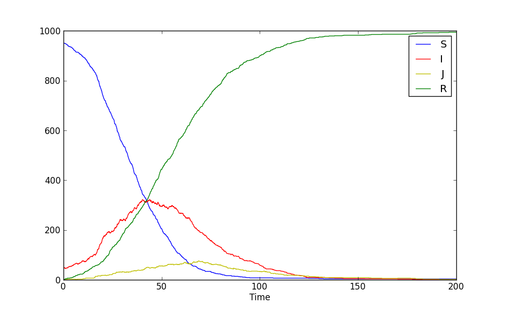
Run it and see how it looks, observe how the system reacts once a few super-spreaders have appeared. This the plot from one of my runs over 2000 iterations (dt = 0.1), with alpha = 0.01 ( and gamma and beta as in the SIR example above), and an initial network with S = 0.95, I = 0.05, J = 0, R = 0:
 now is a function
 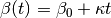 , where
  are parameters but
  is the time the node has been in the I state. Thus the infectiousness of a node increases linearly with the time of infection. Implement this process. Tip: remember that a node may have other attributes than state.